Fourier Series Animation
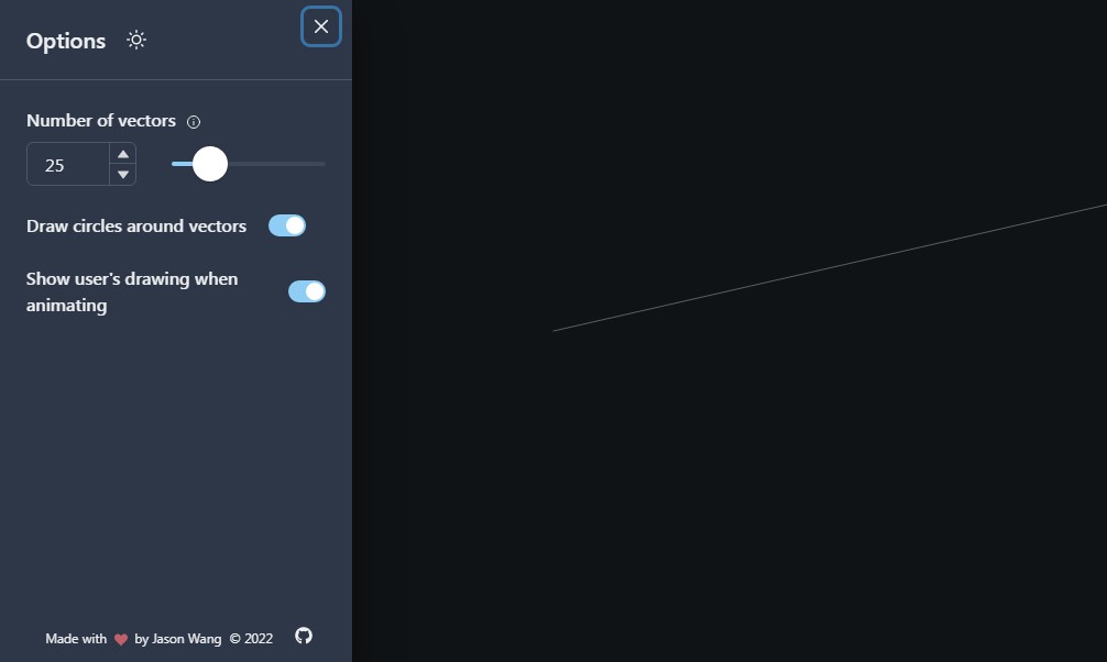
An interactive React web app that demonstrates how an arbitrary user-inputted line drawing can be approximated using the Fourier series. The concept is modelled through the visualisation of rotating vectors put end-to-end, with the Fourier series being used to determine the magnitude and initial position of each vector.
Inspired by 3Blue1Brown’s video explaining and demonstrating the topic
Usage
Try it out directly here: https://jasonfyw.com/fourier-series/
Or clone it onto your own machine
$ git clone https://github.com/jasonfyw/fourier-series
Install the dependencies
$ cd fourier-series
$ npm install
And then start the development server
$ npm start
About the Fourier series
The Fourier series is a branch of Fourier analysis that aims to decompose a periodic function into a sum of exponentials (or trigonometric functions) with different frequencies and magnitudes. This is where the concept of rotating vectors placed end-to-end tracing out a function is derived.
Being able to do this allows for an arbitrary periodic function to be broken up into discrete terms that can then be easily manipulate. As a result, it has a lot of applications in physics such as with signal/image processing, quantum physics, electrical engineering and more.
In this particular demonstration, we are defining $f(t)$ to be a periodic complex function with $t\in[0, 1]$. The exact data points in the codomain are given by a user-drawn input which are then mapped to the domain.
The essential idea is to represent $f(t)$ as a sum of exponential functions rotating at frequencies of $0, 1, -1, 2, -2, …$ rotations per $t$. Each of these exponential functions will be multiplied by a complex coefficient, $c_n$ (where $n$ is the frequency), to determine its initial position and magnitude:
$$ f(t) = \dots + c_{-2}e^{-2\cdot 2\pi it} + c_{-1}e^{-1\cdot 2\pi it} + c_{0}e^{0\cdot 2\pi it} + c_{1}e^{1\cdot 2\pi it} + c_{2}e^{2\cdot 2\pi it} + \dots $$
The term for the vector that doesn’t rotate at all is $c_0$. This can be though of as the ‘centre’ of the whole function – or the average of all the points in the function. This can be computed by taking the integral of the function across its domain:
$$ \int_0^1 f(t) dt $$
By expanding $f(t)$ in terms of its Fourier series:
$$ \int_0^1 f(t) dt = \int_0^1 (\dots + c_{-1}e^{-1\cdot 2\pi it} + c_{0}e^{0\cdot 2\pi it} + c_{1}e^{1\cdot 2\pi it} + \dots)dt $$
and then distributing the definite integral:
$$ \int_0^1 f(t) dt = \dots + \int_0^1c_{-1}e^{-1\cdot 2\pi it}dt + \int_0^1c_{0}e^{0\cdot 2\pi it}dt + \int_0^1c_{1}e^{1\cdot 2\pi it}dt + \dots $$
Every term except for the one with $c_0$ represents the average of a vector that makes a whole number of rotations, which cancel to zero. Hence,
$$ \int_0^1 f(t) dt = \dots + 0 + c_0 + 0 + \dots = c_0 $$
This yields the value for $c_0$.
For an arbitrary coefficient $c_n$, the integral above can be modified by multiplying $f(t)$ by the term $e^{-n2\pi it}$:
$$ \int_0^1 f(t)e^{-n2\pi it} dt $$
Upon expanding $f(t)$ and distributing the exponential term,
$$ \int_0^1 f(t)e^{-n2\pi it} dt = \int_0^1 (\dots + c_{0}e^{-2\cdot 2\pi it} + c_{1}e^{-1\cdot 2\pi it} + \dots + c_{n}e^{0\cdot 2\pi it} + \dots)dt $$
Now, every term apart from that with $c_n$ is an average over vectors that rotate a whole number of turns, which cancels out to zero. This leaves just the $c_n$ term remianing, resulting in the following generalised expression to find any arbitrary $c_n$:
$$ c_n = \int_0^1 f(t)e^{-n2\pi it} dt $$
In this implementation, the program performs the computation numerically to find the Fourier series of an inputted function to a certain number of terms. For an exact representation of the original function, there would have to be infinitely many terms.
Using the computed coefficients, the program plots the resulting approximation of the function.